Including NXB with multi-response
Including the contribution of NXB is easy to do using the multiresponse interface of PyXSPEC. We explore this using a mock X-IFU observation of a galaxy cluster.
Data loading with PyXSPEC
Let's first load the data and define our observational configuration.
import os
import xspec

xspec.AllData.clear()
xspec.AllModels.clear()

# Some settings for XSPEC
xspec.Fit.statMethod = "cstat"
xspec.Fit.bayes = "off"
xspec.Xset.xsect = "vern"
xspec.Xset.abund = "wilm"

xspec_observation = xspec.Spectrum(
    "fakeit_A85.pha",
    respFile="ABELL85_CORE_60k_60k_Hp_allpix_L.rmf"
    arfFile="xa201099010rsl_p0px1000_ptsrc.arf"
)

# Removing bad channels
xspec.AllData.ignore("bad")

# Set the energy band
low_energy, high_energy = 1.5, 8.
xspec_observation.ignore(f"0.0-{low_energy:.1f} {high_energy:.1f}-**")
Models
Now, we define the model for the cluster as a simple absorbed and broadened APEC model.
cluster_model = xspec.Model("tbabs*bapec", sourceNum = 1, modName = 'cluster')
cluster_model.show()
Now, we can define the multi-response for the NXB. As the NXB is contributed by the instrument solely, it doesn't go through the effective area. Hence, we define the multi-response as follows.
xspec_observation.multiresponse[1] = xspec_observation.multiresponse[0].rmf
nxb_model = xspec.Model("pow", sourceNum = 2, modName = 'nxb', setPars={1:0,2:1e-5})
nxb_model.show()
Prior distributions
Now, there are subtle differences when interacting with a multi-model and a single model. For instance, we have to explicitly state which model correspond to which parameter. In particular, note that the prior tuple are in the form (modelName, componentName, parameterName, distribution) instead of (componentName, parameterName, distribution).
from bsixsa.priors import uniform, loguniform

xspec.AllModels(1, modName="cluster").TBabs.nH = "0.01, -1, 0, 0, 1, 1"
xspec.AllModels(1, modName="nxb").powerlaw.PhoIndex = "0., -1, 0, 0, 1, 1"

prior = [
    ("cluster", "bapec", "kT", uniform(0, 7)),
    ("cluster", "bapec", "Abundanc", uniform(0, 4)),
    ("cluster", "bapec", "Redshift", uniform(0.05, 0.3)),
    ("cluster", "bapec", "Velocity", uniform(0.5, 1000)),
    ("cluster", "bapec", "norm", loguniform(1e-5, 1e-2)),
    ("nxb", "powerlaw", "norm", loguniform(1e-4, 1e0)),
]
Solver
Once this is set, we can fit the data.
from bsixsa import Solver, Nessai

solver = Solver(
    prior,
    outputfiles_basename="result_nessai_nxb/",
    overwrite=True,
    backend=Nessai()
)
As in the other fits, we should first check if the priors are properly chosen.
solver.plot_predictive_coverage(
    "prior",
    residual_kind="sigma",
    grouping=30,
    figsize=(7,5),
    y_lim=(2, 5e7)
);
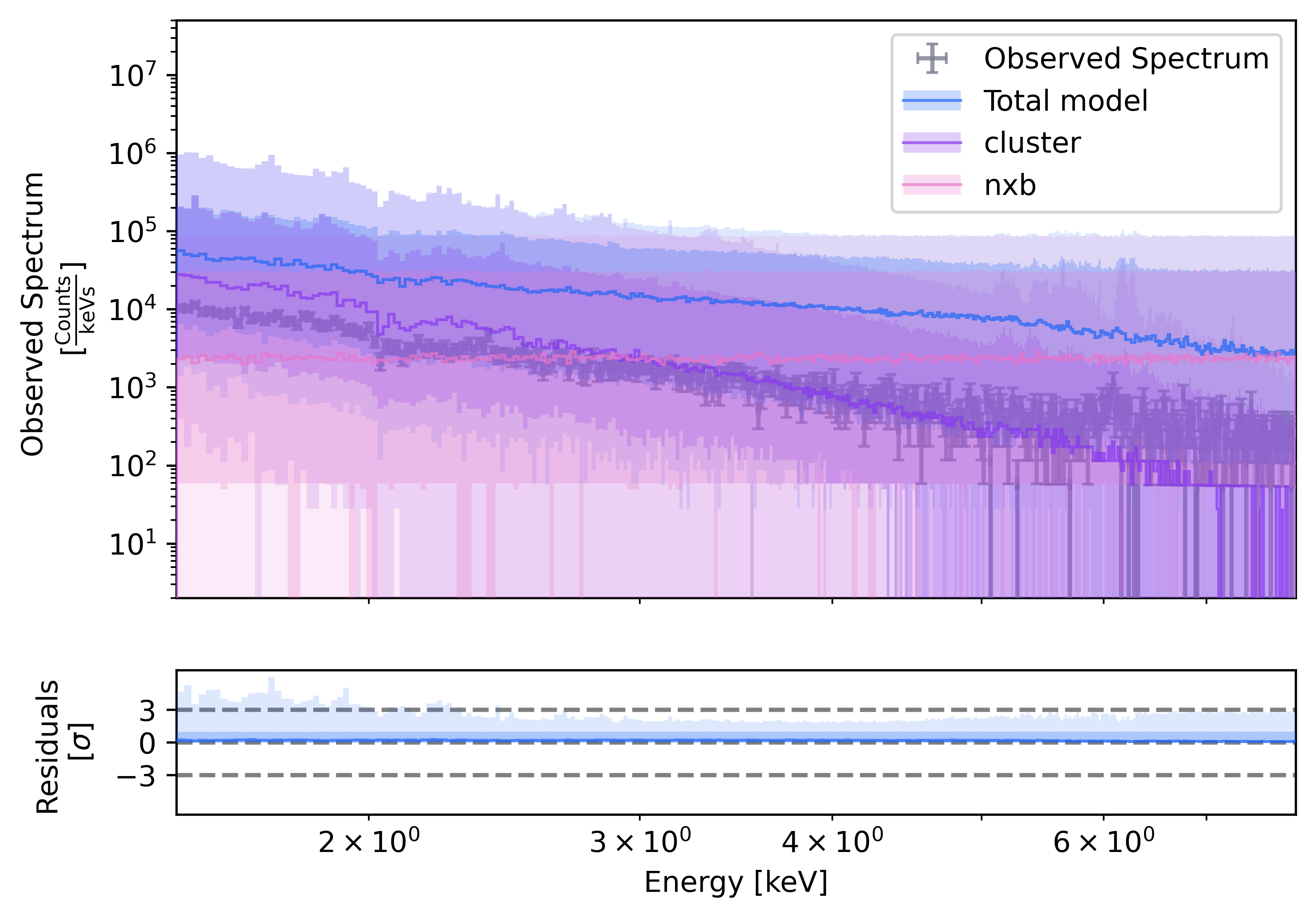
Prior predictive coverage for the configured model and priors.
Let's run the sampler.
fit_result = solver.run()
Now, the fit should be good! Let's check the posterior predictive.
solver.plot_predictive_coverage(
    "posterior",
    residual_kind="sigma",
    grouping=30,
    figsize=(7,5),
    y_lim=(1e2, 3e4)
);
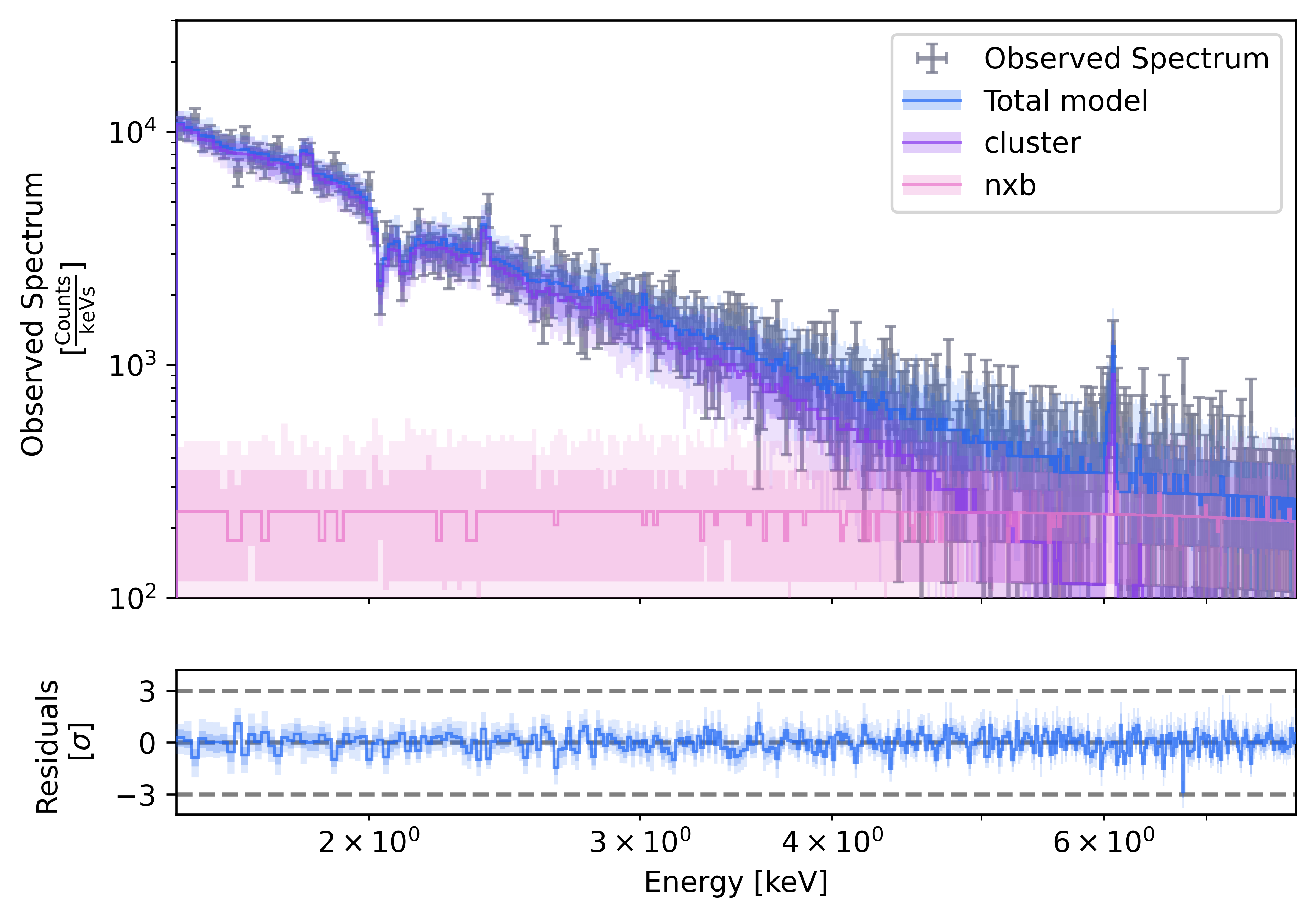
Posterior predictive coverage after running the nested sampler.