Simple fit
This page walks through a complete fit that is representative of the Tycho SNR analysis as seen by Chandra/ACIS, from loading OGIP files with PyXSPEC to checking the posterior predictive coverage. The snippets are meant to be read in order: each block builds on the objects created in the previous one.
Data loading with PyXSPEC
Start by importing PyXSPEC, clearing any state left from a previous interactive session, and setting the XSPEC options used for this fit.
import os
import xspec

xspec.AllData.clear()
xspec.AllModels.clear()

# Some settings for XSPEC
xspec.Fit.statMethod = "cstat"
xspec.Fit.bayes = "off"
xspec.Xset.xsect = "vern"
xspec.Xset.abund = "lpgs"
Next, let's load the source spectrum together with its response files. Once the data are loaded, we ignore the bad channels and restrict the fit to the energy band of interest.
xspec_observation = xspec.Spectrum(
    "fakeit_tycho_raw.pha",
    respFile="reg_64_10093.rmf",
    arfFile="reg_64_10093.arf",
)

# Removing bad channels
xspec.AllData.ignore("bad")

# Set the energy band
low_energy, high_energy = 0.5, 10.
xspec_observation.ignore(f"0.0-{low_energy:.1f} {high_energy:.1f}-**")
With the data in place, define the spectral model that will be sampled. Here the absorption component multiplies two vnei plasma components, which lets the fit capture multiple thermal populations.
xspec.Xset.addModelString("NEIAPECROOT","3.1.3") # Extra model variable
xspec_model = xspec.Model("tbabs*(vnei + vnei)")
xspec_model.show()
Prior distributions
The next block freezes or constrains the PyXSPEC parameters and then declares the priors for the parameters that will actually be sampled. Every parameter must be either frozen (by setting its error to a negative value) or set to a prior distribution.
from bsixsa.priors import uniform, loguniform
from bsixsa.convenience import XSilence

with XSilence():

    # We apologize for this heavy syntax, this is directly inherited from pyXSPEC

    xspec_model.vnei_3.Redshift.link = xspec_model.vnei.Redshift

    xspec_model.TBabs.nH = '0.7,-1,0,0,9999,9999'
    # 'value,error,hard_low,soft_low,soft_high,hard_high'
    # Error set to negative value tells XSPEC to keep it frozen during the fit

    xspec_model.vnei.H = '1,-1,0,0,9999,9999'
    xspec_model.vnei.He = '1,-1,0,0,9999,9999'
    xspec_model.vnei.C = '1,-1,0,0,9999,9999'
    xspec_model.vnei.N = '1,-1,0,0,9999,9999'
    xspec_model.vnei.O = '1,-1,0,0,9999,9999'
    xspec_model.vnei.Ne = '1,-1,0,0,9999,9999'
    xspec_model.vnei.Fe = '1,-1,0,0,9999,9999'
    xspec_model.vnei.Ni = '1,-1,0,0,9999,9999'
    xspec_model.vnei.Ca = '1750,-1,0,0,9999,9999'
    xspec_model.vnei.Tau = '4.7e10,-1,0,0,1e11,1e11'
    xspec_model.vnei.Redshift = '0,-1,-1,-1,1,1'
    xspec_model.vnei.norm = '7e-6,-1,0,0,1,1'

    xspec_model.vnei_3.H = '1,-1,0,0,9999,9999'
    xspec_model.vnei_3.He = '1,-1,0,0,9999,9999'
    xspec_model.vnei_3.C = '1,-1,0,0,9999,9999'
    xspec_model.vnei_3.N = '1,-1,0,0,9999,9999'
    xspec_model.vnei_3.O = '1,-1,0,0,9999,9999'
    xspec_model.vnei_3.Ne = '1,-1,0,0,9999,9999'
    xspec_model.vnei_3.Mg = '1000,-1,0,0,9999,9999'
    xspec_model.vnei_3.Si = '1000,-1,0,0,9999,9999'
    xspec_model.vnei_3.S = '1,-1,0,0,9999,9999'
    xspec_model.vnei_3.Ar = '1,-1,0,0,9999,9999'
    xspec_model.vnei_3.Ca = '1,-1,0,0,9999,9999'
    xspec_model.vnei_3.Si = '1000,-1,0,0,9999,9999'

prior = [
    ("vnei_2", "kT", uniform(0.4, 5.)),
    ("vnei_2", "Mg", loguniform(0.1, 500.)),
    ("vnei_2", "Si", loguniform(50., 5_000.)),
    ("vnei_2", "S", loguniform(50., 5_000.)),
    ("vnei_2", "Ar", loguniform(50., 5_000.)),
    ("vnei_2", "Tau", loguniform(5e8, 5e11)),
    ("vnei_2", "Redshift", uniform(-6e-2, +6e-2)),
    ("vnei_2", "norm", loguniform(1e-7, 1e-3)),
    ("vnei_3", "kT", uniform(5., 20.)),
    ("vnei_3", "Fe", loguniform(50., 5_000.)),
    ("vnei_3", "Tau", loguniform(5e8, 5e11)),
    ("vnei_3", "norm", loguniform(1e-8, 1e-4)),
]
Solver
Once the priors are ready, instantiate the solver. This object coordinates everything needed to run the inference, and the backend is inferred from the BackendConfig passed at construction time.
from bsixsa import Solver, Nautilus

solver = Solver(
    prior,
    outputfiles_basename="result/",
    overwrite=True,
    backend=Nautilus(num_live_points=2_000),
)
Before launching the fit, it is essential to check whether the prior alone generates spectra that are compatible with the observed counts. Large mismatches here often indicate that a bound or model assumption should be revisited.
solver.plot_predictive_coverage("prior", min_counts=10, residual_kind="sigma", figsize=(7,5));
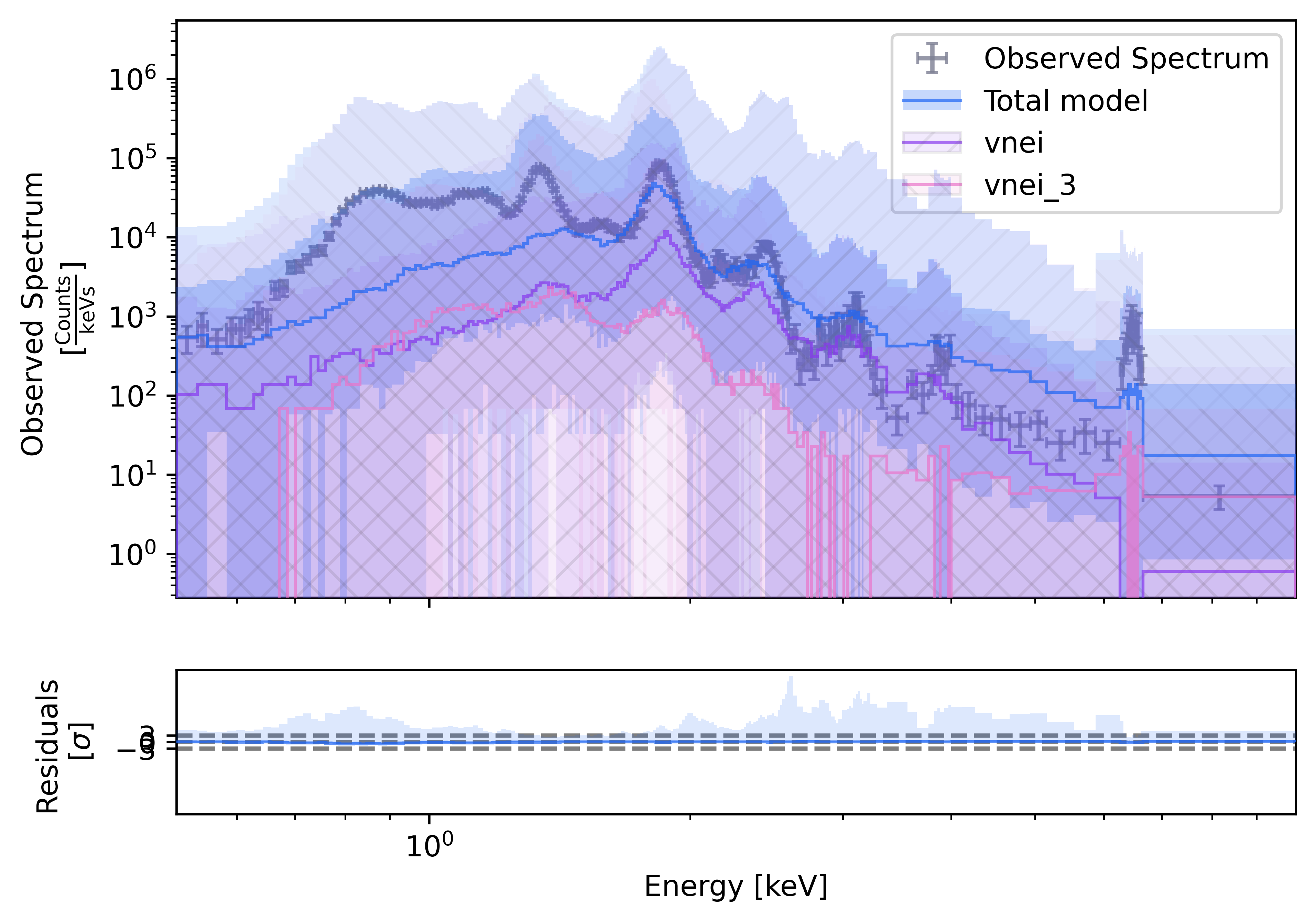
Prior predictive coverage for the configured model and priors.
As the prior predictive check looks reasonable, we run the sampler.
fit_result = solver.run()
After sampling, compare posterior predictive spectra with the data. This is the quickest visual check that the fitted model explains the observed counts and residual structure.
solver.plot_predictive_coverage("posterior", min_counts=10, residual_kind="sigma", figsize=(7,5));
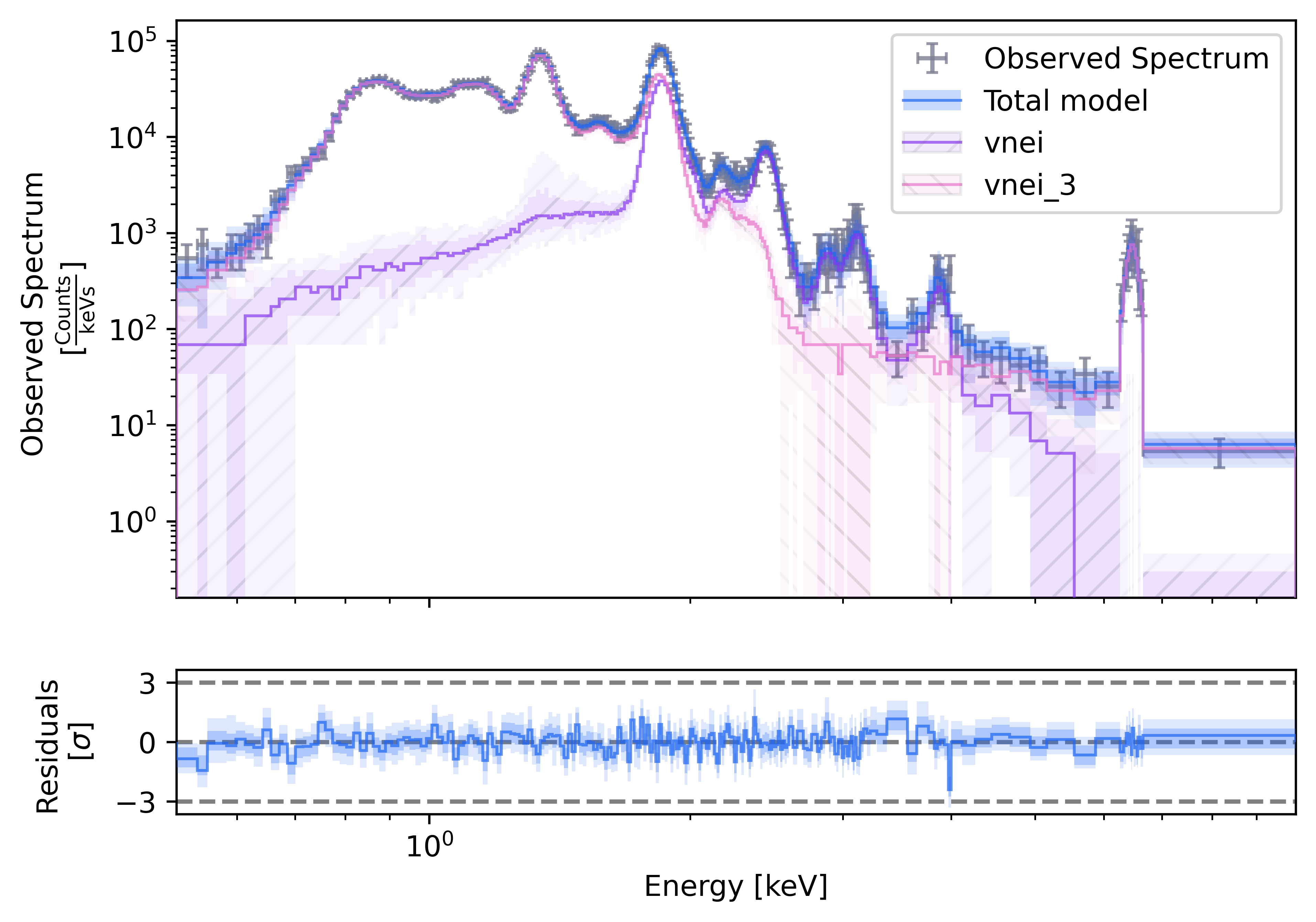
Posterior predictive coverage after running the nested sampler.